तीव्रतम अवतरण की विधि: Difference between revisions
(Created page with "{{Short description|Extension of Laplace's method for approximating integrals}} {{for|the optimization algorithm|Gradient descent}} गणित में, तीव्रत...") |
No edit summary |
||
| Line 12: | Line 12: | ||
== मूल विचार == | == मूल विचार == | ||
तीव्रतम अवतरण की विधि प्रपत्र के एक जटिल अभिन्न अंग का अनुमान लगाने की एक विधि है<math display="block">I(\lambda) = \int_Cf(z)e^{\lambda g(z)}\,\mathrm{d}z</math>बड़े के लिए <math>\lambda \rightarrow \infty</math>, कहाँ <math>f(z)</math> और <math>g(z)</math> के [[विश्लेषणात्मक कार्य]] हैं <math>z</math>. क्योंकि इंटीग्रैंड विश्लेषणात्मक है, रूपरेखा <math>C</math> एक नये स्वरूप में विकृत किया जा सकता है <math>C'</math> अभिन्न को बदले बिना. विशेष रूप से, कोई एक नई रूपरेखा की तलाश करता है जिस पर काल्पनिक भाग हो <math>g(z) = \text{Re} [g(z)] + i \, \text{Im}[g(z)]</math> स्थिर है. तब <math display="block">I(\lambda) = e^{i \lambda \text{Im}\{g(z)\}} \int_{C'}f(z)e^{\lambda \text{Re} \{g(z)\}}\,\mathrm{d}z,</math>और शेष अभिन्न का अनुमान लाप्लास की विधि जैसी अन्य विधियों से लगाया जा सकता है।<ref>{{Cite book|last1=Bender|first1=Carl M.|url=http://link.springer.com/10.1007/978-1-4757-3069-2|title=वैज्ञानिकों और इंजीनियरों के लिए उन्नत गणितीय तरीके I|last2=Orszag|first2=Steven A.|date=1999|publisher=Springer New York|isbn=978-1-4419-3187-0|location=New York, NY|language=en|doi=10.1007/978-1-4757-3069-2}}</ref> | तीव्रतम अवतरण की विधि प्रपत्र के एक जटिल अभिन्न अंग का अनुमान लगाने की एक विधि है<math display="block">I(\lambda) = \int_Cf(z)e^{\lambda g(z)}\,\mathrm{d}z</math>बड़े के लिए <math>\lambda \rightarrow \infty</math>, कहाँ <math>f(z)</math> और <math>g(z)</math> के [[विश्लेषणात्मक कार्य]] हैं <math>z</math>. क्योंकि इंटीग्रैंड विश्लेषणात्मक है, रूपरेखा <math>C</math> एक नये स्वरूप में विकृत किया जा सकता है <math>C'</math> अभिन्न को बदले बिना. विशेष रूप से, कोई एक नई रूपरेखा की तलाश करता है जिस पर काल्पनिक भाग हो <math>g(z) = \text{Re} [g(z)] + i \, \text{Im}[g(z)]</math> स्थिर है. तब<math display="block">I(\lambda) = e^{i \lambda \text{Im}\{g(z)\}} \int_{C'}f(z)e^{\lambda \text{Re} \{g(z)\}}\,\mathrm{d}z,</math>और शेष अभिन्न का अनुमान लाप्लास की विधि जैसी अन्य विधियों से लगाया जा सकता है।<ref>{{Cite book|last1=Bender|first1=Carl M.|url=http://link.springer.com/10.1007/978-1-4757-3069-2|title=वैज्ञानिकों और इंजीनियरों के लिए उन्नत गणितीय तरीके I|last2=Orszag|first2=Steven A.|date=1999|publisher=Springer New York|isbn=978-1-4419-3187-0|location=New York, NY|language=en|doi=10.1007/978-1-4757-3069-2}}</ref> | ||
== व्युत्पत्ति == | == व्युत्पत्ति == | ||
| Line 25: | Line 24: | ||
= | = | ||
- \frac{\partial Y}{\partial x} | - \frac{\partial Y}{\partial x} | ||
.</math>तब <math display="block">\frac{\partial X}{\partial x} \frac{\partial Y}{\partial x} + \frac{\partial X}{\partial y} \frac{\partial Y}{\partial y} = \nabla X \cdot \nabla Y = 0,</math>इसलिए स्थिर चरण की आकृतियाँ भी तीव्रतम अवतरण की आकृतियाँ हैं। | .</math>तब<math display="block">\frac{\partial X}{\partial x} \frac{\partial Y}{\partial x} + \frac{\partial X}{\partial y} \frac{\partial Y}{\partial y} = \nabla X \cdot \nabla Y = 0,</math>इसलिए स्थिर चरण की आकृतियाँ भी तीव्रतम अवतरण की आकृतियाँ हैं। | ||
==एक साधारण अनुमान== | ==एक साधारण अनुमान== | ||
| Line 44: | Line 43: | ||
&= \underbrace{e^{-\lambda_0 M} \int_{C} \left| f(x) e^{\lambda_0 S(x)} \right| dx}_{\text{const}} \cdot e^{\lambda M}. | &= \underbrace{e^{-\lambda_0 M} \int_{C} \left| f(x) e^{\lambda_0 S(x)} \right| dx}_{\text{const}} \cdot e^{\lambda M}. | ||
\end{align}</math> | \end{align}</math> | ||
== एकल गैर-क्षतिग्रस्त काठी बिंदु का मामला == | == एकल गैर-क्षतिग्रस्त काठी बिंदु का मामला == | ||
| Line 153: | Line 151: | ||
If <math>\det \boldsymbol{\varphi}'_w(0) = -1</math>, then interchanging two variables assures that <math>\det \boldsymbol{\varphi}'_w(0) = +1</math>. | If <math>\det \boldsymbol{\varphi}'_w(0) = -1</math>, then interchanging two variables assures that <math>\det \boldsymbol{\varphi}'_w(0) = +1</math>. | ||
}} | }}'''एकल गैर-पतित काठी बिंदु के मामले में स्पर्शोन्मुख विस्तार''' | ||
मान लीजिए | मान लीजिए | ||
# {{math| ''f'' (''z'')}} और {{math|''S''(''z'')}} [[ खुला सेट ]], बाउंडेड सेट (टोपोलॉजिकल वेक्टर स्पेस) और [[ बस जुड़ा हुआ स्थान ]] सेट में होलोमोर्फिक फ़ंक्शन फ़ंक्शन हैं {{math|Ω''<sub>x</sub>'' ⊂ '''C'''<sup>''n''</sup>}} ऐसा कि {{math|''I<sub>x</sub>'' {{=}} Ω''<sub>x</sub>'' ∩ '''R'''<sup>''n''</sup>}} [[ जुड़ा हुआ स्थान ]] है; | # {{math| ''f'' (''z'')}} और {{math|''S''(''z'')}} [[ खुला सेट ]], बाउंडेड सेट (टोपोलॉजिकल वेक्टर स्पेस) और [[ बस जुड़ा हुआ स्थान ]] सेट में होलोमोर्फिक फ़ंक्शन फ़ंक्शन हैं {{math|Ω''<sub>x</sub>'' ⊂ '''C'''<sup>''n''</sup>}} ऐसा कि {{math|''I<sub>x</sub>'' {{=}} Ω''<sub>x</sub>'' ∩ '''R'''<sup>''n''</sup>}} [[ जुड़ा हुआ स्थान ]] है; | ||
| Line 188: | Line 183: | ||
:<math>\mathcal{I}_j = \frac{2}{\sqrt{-\mu_j}\sqrt{\lambda}} \int_0^{\infty} e^{-\frac{\xi^2}{2}} d\xi = \sqrt{\frac{2\pi}{\lambda}} (-\mu_j)^{-\frac{1}{2}}.</math> | :<math>\mathcal{I}_j = \frac{2}{\sqrt{-\mu_j}\sqrt{\lambda}} \int_0^{\infty} e^{-\frac{\xi^2}{2}} d\xi = \sqrt{\frac{2\pi}{\lambda}} (-\mu_j)^{-\frac{1}{2}}.</math> | ||
}} | }} | ||
समीकरण (8) को इस प्रकार भी लिखा जा सकता है{{NumBlk|:|<math>I(\lambda) = \left( \frac{2\pi}{\lambda}\right)^{\frac{n}{2}} e^{\lambda S(x^0)} \left ( \det (-S_{xx}''(x^0)) \right )^{-\frac{1}{2}} \left (f(x^0) + O\left(\lambda^{-1}\right) \right),</math>|{{EquationRef|13}}}} | |||
समीकरण (8) को इस प्रकार भी लिखा जा सकता है | |||
{{NumBlk|:|<math>I(\lambda) = \left( \frac{2\pi}{\lambda}\right)^{\frac{n}{2}} e^{\lambda S(x^0)} \left ( \det (-S_{xx}''(x^0)) \right )^{-\frac{1}{2}} \left (f(x^0) + O\left(\lambda^{-1}\right) \right),</math>|{{EquationRef|13}}}} | |||
की शाखा कहां है | की शाखा कहां है | ||
| Line 261: | Line 253: | ||
{{reflist}} | {{reflist}} | ||
== संदर्भ == | |||
==संदर्भ== | |||
*{{Citation | *{{Citation | ||
| last1=Chaichian | | last1=Chaichian | ||
Revision as of 17:57, 4 December 2023
गणित में, तीव्रतम अवतरण या काठी-बिंदु विधि की विधि एक इंटीग्रल का अनुमान लगाने के लिए लाप्लास की विधि का एक विस्तार है, जहां एक स्थिर बिंदु (सैडल बिंदु) के पास से गुजरने के लिए जटिल विमान में एक समोच्च इंटीग्रल को विकृत किया जाता है, मोटे तौर पर दिशा में तीव्रतम अवतरण या स्थिर चरण। सैडल-पॉइंट सन्निकटन का उपयोग जटिल विमान में इंटीग्रल्स के साथ किया जाता है, जबकि लाप्लास की विधि का उपयोग वास्तविक इंटीग्रल्स के साथ किया जाता है।
अनुमान लगाया जाने वाला अभिन्न अंग अक्सर रूप का होता है
जहां C एक समोच्च है, और λ बड़ा है। सबसे तेज वंश की विधि का एक संस्करण एकीकरण सी के समोच्च को एक नए पथ एकीकरण सी' में विकृत कर देता है ताकि निम्नलिखित स्थितियाँ बनी रहें:
- C′ व्युत्पन्न g′(z) के एक या अधिक शून्य से होकर गुजरता है,
- g(z) का काल्पनिक भाग C′ पर स्थिर है।
तीव्रतम अवतरण की विधि सबसे पहले किसके द्वारा प्रकाशित की गई थी? Debye (1909), जिन्होंने बेसेल कार्यों का अनुमान लगाने के लिए इसका उपयोग किया और बताया कि यह अप्रकाशित नोट में हुआ था Riemann (1863)हाइपरज्यामितीय कार्य के बारे में। सबसे तीव्र ढलान के समोच्च में न्यूनतम गुण होता है, देखें Fedoryuk (2001). Siegel (1932) रीमैन के कुछ अन्य अप्रकाशित नोट्स का वर्णन किया, जहां उन्होंने रीमैन-सीगल फॉर्मूला प्राप्त करने के लिए इस विधि का उपयोग किया।
मूल विचार
तीव्रतम अवतरण की विधि प्रपत्र के एक जटिल अभिन्न अंग का अनुमान लगाने की एक विधि है
व्युत्पत्ति
विश्लेषणात्मक होने के कारण इस विधि को तीव्रतम अवतरण की विधि कहा जाता है , स्थिर चरण समोच्च तीव्रतम अवरोही समोच्चों के समतुल्य हैं।
अगर का एक विश्लेषणात्मक कार्य है , यह कॉची-रीमैन समीकरण को संतुष्ट करता है
एक साधारण अनुमान
होने देना f, S : Cn → C और C ⊂ Cn. अगर
कहाँ वास्तविक भाग को दर्शाता है, और एक सकारात्मक वास्तविक संख्या मौजूद है λ0 ऐसा है कि
तो निम्नलिखित अनुमान मान्य है:[2]
सरल अनुमान का प्रमाण:
एकल गैर-क्षतिग्रस्त काठी बिंदु का मामला
मूल धारणाएँ और संकेतन
होने देना x एक जटिल हो n-आयामी वेक्टर, और
किसी फ़ंक्शन के लिए हेस्सियन मैट्रिक्स को निरूपित करें S(x). अगर
एक वेक्टर फ़ंक्शन है, तो इसके जैकोबियन मैट्रिक्स और निर्धारक को इस प्रकार परिभाषित किया गया है
एक गैर पतित काठी बिंदु, z0 ∈ Cn, एक होलोमोर्फिक फ़ंक्शन का S(z) फ़ंक्शन का एक महत्वपूर्ण बिंदु है (यानी, ∇S(z0) = 0) जहां फ़ंक्शन के हेसियन मैट्रिक्स में एक गैर-लुप्त होने वाला निर्धारक है (यानी, ).
गैर-अपक्षयी सैडल बिंदु के मामले में इंटीग्रल के एसिम्प्टोटिक्स के निर्माण के लिए निम्नलिखित मुख्य उपकरण है:
कॉम्प्लेक्स मोर्स लेम्मा
वास्तविक-मूल्यवान कार्यों के लिए मोर्स सिद्धांत#मोर्स लेम्मा निम्नानुसार सामान्यीकृत होता है[3] होलोमोर्फिक फ़ंक्शन के लिए: एक गैर-पतित काठी बिंदु के पास z0 एक होलोमोर्फिक फ़ंक्शन का S(z), जिसके संदर्भ में निर्देशांक मौजूद हैं S(z) − S(z0) बिल्कुल द्विघात है. इसे सटीक बनाने के लिए आइए Sडोमेन के साथ एक होलोमोर्फिक फ़ंक्शन बनें W ⊂ Cn, और जाने z0 में W का एक गैर पतित काठी बिंदु हो S, वह है, ∇S(z0) = 0 और . फिर पड़ोस मौजूद हैं U ⊂ W का z0 और V ⊂ Cn का w = 0, और एक वन-टू-वन फ़ंक्शन होलोमोर्फिक फ़ंक्शन φ : V → U साथ φ(0) = z0 ऐसा है कि
यहां ही μj मैट्रिक्स के आइगेनवैल्यूज़ एवं आइगेनवेक्टर्स हैं .
फ़ाइल:कॉम्प्लेक्स मोर्स लेम्मा चित्रण.पीडीएफ|अंगूठे|केंद्र
The following proof is a straightforward generalization of the proof of the real Morse Lemma, which can be found in.[4] We begin by demonstrating
- Auxiliary statement. Let f : Cn → C be holomorphic in a neighborhood of the origin and f (0) = 0. Then in some neighborhood, there exist functions gi : Cn → C such that where each gi is holomorphic and
From the identity
we conclude that
and
Without loss of generality, we translate the origin to z0, such that z0 = 0 and S(0) = 0. Using the Auxiliary Statement, we have
Since the origin is a saddle point,
we can also apply the Auxiliary Statement to the functions gi(z) and obtain
-
(1)
Recall that an arbitrary matrix A can be represented as a sum of symmetric A(s) and anti-symmetric A(a) matrices,
The contraction of any symmetric matrix B with an arbitrary matrix A is
-
(2)
i.e., the anti-symmetric component of A does not contribute because
Thus, hij(z) in equation (1) can be assumed to be symmetric with respect to the interchange of the indices i and j. Note that
hence, det(hij(0)) ≠ 0 because the origin is a non-degenerate saddle point.
Let us show by induction that there are local coordinates u = (u1, ... un), z = ψ(u), 0 = ψ(0), such that
-
(3)
First, assume that there exist local coordinates y = (y1, ... yn), z = φ(y), 0 = φ(0), such that
-
(4)
where Hij is symmetric due to equation (2). By a linear change of the variables (yr, ... yn), we can assure that Hrr(0) ≠ 0. From the chain rule, we have
Therefore:
whence,
The matrix (Hij(0)) can be recast in the Jordan normal form: (Hij(0)) = LJL−1, were L gives the desired non-singular linear transformation and the diagonal of J contains non-zero eigenvalues of (Hij(0)). If Hij(0) ≠ 0 then, due to continuity of Hij(y), it must be also non-vanishing in some neighborhood of the origin. Having introduced , we write
Motivated by the last expression, we introduce new coordinates z = η(x), 0 = η(0),
The change of the variables y ↔ x is locally invertible since the corresponding Jacobian is non-zero,
Therefore,
-
(5)
Comparing equations (4) and (5), we conclude that equation (3) is verified. Denoting the eigenvalues of by μj, equation (3) can be rewritten as
-
(6)
Therefore,
-
(7)
From equation (6), it follows that . The Jordan normal form of reads , where Jz is an upper diagonal matrix containing the eigenvalues and det P ≠ 0; hence, . We obtain from equation (7)
If , then interchanging two variables assures that .
एकल गैर-पतित काठी बिंदु के मामले में स्पर्शोन्मुख विस्तार
मान लीजिए
- f (z) और S(z) खुला सेट , बाउंडेड सेट (टोपोलॉजिकल वेक्टर स्पेस) और बस जुड़ा हुआ स्थान सेट में होलोमोर्फिक फ़ंक्शन फ़ंक्शन हैं Ωx ⊂ Cn ऐसा कि Ix = Ωx ∩ Rn जुड़ा हुआ स्थान है;
- एक एकल अधिकतम है: बिल्कुल एक बिंदु के लिए x0 ∈ Ix;
- x0 एक गैर-पतित काठी बिंदु है (यानी, ∇S(x0) = 0 और ).
फिर, निम्नलिखित स्पर्शोन्मुख धारण करता है
-
(8)
कहाँ μj हेस्सियन मैट्रिक्स के eigenvalues हैं और तर्कों से परिभाषित किये गये हैं
-
(9)
यह कथन फेडोर्युक (1987) में प्रस्तुत अधिक सामान्य परिणामों का एक विशेष मामला है।[5]
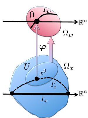
First, we deform the contour Ix into a new contour passing through the saddle point x0 and sharing the boundary with Ix. This deformation does not change the value of the integral I(λ). We employ the Complex Morse Lemma to change the variables of integration. According to the lemma, the function φ(w) maps a neighborhood x0 ∈ U ⊂ Ωx onto a neighborhood Ωw containing the origin. The integral I(λ) can be split into two: I(λ) = I0(λ) + I1(λ), where I0(λ) is the integral over , while I1(λ) is over (i.e., the remaining part of the contour I′x). Since the latter region does not contain the saddle point x0, the value of I1(λ) is exponentially smaller than I0(λ) as λ → ∞;[6] thus, I1(λ) is ignored. Introducing the contour Iw such that , we have
-
(10)
Recalling that x0 = φ(0) as well as , we expand the pre-exponential function into a Taylor series and keep just the leading zero-order term
-
(11)
Here, we have substituted the integration region Iw by Rn because both contain the origin, which is a saddle point, hence they are equal up to an exponentially small term.[7] The integrals in the r.h.s. of equation (11) can be expressed as
-
(12)
From this representation, we conclude that condition (9) must be satisfied in order for the r.h.s. and l.h.s. of equation (12) to coincide. According to assumption 2, is a negatively defined quadratic form (viz., ) implying the existence of the integral , which is readily calculated
समीकरण (8) को इस प्रकार भी लिखा जा सकता है
-
(13)
की शाखा कहां है
निम्नानुसार चुना गया है
महत्वपूर्ण विशेष मामलों पर विचार करें:
- अगर S(x) वास्तविक के लिए वास्तविक मूल्यवान है x और x0 में Rn (उर्फ, बहुआयामी लाप्लास विधि), फिर[8]
- अगर S(x) वास्तव में पूर्णतया काल्पनिक है x (अर्थात।, सभी के लिए x में Rn) और x0 में Rn (उर्फ, बहुआयामी स्थिर चरण विधि),[9] तब[10] कहाँ सिल्वेस्टर के जड़त्व के नियम को दर्शाता है#प्रमेय का कथन , जो नकारात्मक eigenvalues की संख्या घटाकर सकारात्मक लोगों की संख्या के बराबर है। यह उल्लेखनीय है कि क्वांटम यांत्रिकी (साथ ही प्रकाशिकी में) में बहुआयामी WKB सन्निकटन के लिए स्थिर चरण विधि के अनुप्रयोगों में, Ind मास्लोव सूचकांक से संबंधित है, उदाहरण के लिए, Chaichian & Demichev (2001) और Schulman (2005).
एकाधिक गैर-क्षतिग्रस्त काठी बिंदुओं का मामला
यदि फ़ंक्शन S(x) में कई अलग-अलग गैर-पतित काठी बिंदु हैं, यानी,
कहाँ
का एक खुला आवरण है Ωx, तो एकता के विभाजन को नियोजित करके इंटीग्रल एसिम्प्टोटिक की गणना को एकल सैडल बिंदु के मामले में कम कर दिया जाता है। एकता का विभाजन हमें निरंतर कार्यों का एक सेट बनाने की अनुमति देता है ρk(x) : Ωx → [0, 1], 1 ≤ k ≤ K, ऐसा है कि
कहाँ से,
इसलिए जैसे λ → ∞ हमारे पास है:
जहां अंतिम चरण में समीकरण (13) और पूर्व-घातीय फ़ंक्शन का उपयोग किया गया था f (x) कम से कम निरंतर होना चाहिए.
अन्य मामले
कब ∇S(z0) = 0 और , बिंदु z0 ∈ Cn को किसी फ़ंक्शन का डीजेनरेट सैडल पॉइंट कहा जाता है S(z).
के स्पर्शोन्मुख की गणना
कब λ → ∞, f (x) सतत है, और S(z) में एक पतित काठी बिंदु है, यह एक बहुत ही समृद्ध समस्या है, जिसका समाधान काफी हद तक आपदा सिद्धांत पर निर्भर करता है। यहां, आपदा सिद्धांत ने फ़ंक्शन को बदलने के लिए सबसे तेज वंश#कॉम्प्लेक्स मोर्स लेम्मा की विधि को प्रतिस्थापित कर दिया है, जो केवल गैर-पतित मामले में मान्य है। S(z) विहित अभ्यावेदन की भीड़ में से एक में। अधिक जानकारी के लिए देखें, उदाहरणार्थ, Poston & Stewart (1978) और Fedoryuk (1987).
विकृत काठी बिंदुओं वाले इंटीग्रल स्वाभाविक रूप से कास्टिक (प्रकाशिकी) और क्वांटम यांत्रिकी में बहुआयामी डब्ल्यूकेबी सन्निकटन सहित कई अनुप्रयोगों में दिखाई देते हैं।
अन्य मामले जैसे, उदा. f (x) और/या S(x) असंतुलित हैं या जब चरम सीमा पर हैं S(x) एकीकरण क्षेत्र की सीमा पर स्थित है, विशेष देखभाल की आवश्यकता है (देखें, उदाहरण के लिए, Fedoryuk (1987) और Wong (1989)).
विस्तार और सामान्यीकरण
सबसे तीव्र अवतरण विधि का एक विस्तार तथाकथित अरेखीय स्थिर चरण/सबसे तीव्र अवतरण विधि है। यहां, इंटीग्रल के बजाय, किसी को रीमैन-हिल्बर्ट फ़ैक्टराइज़ेशन समस्याओं के स्पर्शोन्मुख समाधानों का मूल्यांकन करने की आवश्यकता है।
जटिल क्षेत्र में एक समोच्च सी को देखते हुए, उस समोच्च पर परिभाषित एक फ़ंक्शन एफ और एक विशेष बिंदु, मान लीजिए अनंत, एक समोच्च सी से दूर एक फ़ंक्शन एम होलोमोर्फिक की तलाश करता है, सी में निर्धारित छलांग के साथ, और अनंत पर दिए गए सामान्यीकरण के साथ। यदि f और इसलिए M अदिश के बजाय आव्यूह हैं तो यह एक ऐसी समस्या है जो सामान्य तौर पर एक स्पष्ट समाधान स्वीकार नहीं करती है।
तब रैखिक स्थिर चरण/सबसे तीव्र वंश विधि की तर्ज पर एक स्पर्शोन्मुख मूल्यांकन संभव है। विचार यह है कि दी गई रीमैन-हिल्बर्ट समस्या के समाधान को असम्बद्ध रूप से कम करके एक सरल, स्पष्ट रूप से हल करने योग्य, रीमैन-हिल्बर्ट समस्या बना दिया जाए। कॉची के प्रमेय का उपयोग जम्प समोच्च की विकृतियों को उचित ठहराने के लिए किया जाता है।
रूसी गणितज्ञ अलेक्जेंडर इट्स के पहले के काम के आधार पर, 1993 में डेफ्ट और झोउ द्वारा नॉनलाइनियर स्थिर चरण की शुरुआत की गई थी। लैक्स, लीवरमोर, डेफ्ट, वेनाकिड्स और झोउ के पिछले काम के आधार पर, 2003 में कामविसिस, के. मैकलॉघलिन और पी. मिलर द्वारा एक (ठीक से कहें तो) नॉनलाइनियर स्टीपेस्ट डीसेंट विधि पेश की गई थी। जैसा कि रैखिक मामले में होता है, सबसे तीव्र अवरोही आकृतियाँ न्यूनतम-अधिकतम समस्या का समाधान करती हैं। अरैखिक मामले में वे एस-वक्र बन जाते हैं (80 के दशक में स्टाल, गोन्चर और राखमनोव द्वारा एक अलग संदर्भ में परिभाषित)।
नॉनलाइनियर स्थिर चरण/सबसे तेज वंश विधि में सॉलिटन समीकरणों और एकीकृत मॉडल , यादृच्छिक मैट्रिक्स और साहचर्य के सिद्धांत के अनुप्रयोग हैं।
एक अन्य विस्तार काठी बिंदुओं और एकसमान स्पर्शोन्मुख विस्तारों को संयोजित करने के लिए चेस्टर-फ़्रीडमैन-उर्सेल की विधि है।
यह भी देखें
- पियर्सी इंटीग्रल
- स्थिर चरण सन्निकटन
- लाप्लास की विधि
टिप्पणियाँ
- ↑ Bender, Carl M.; Orszag, Steven A. (1999). वैज्ञानिकों और इंजीनियरों के लिए उन्नत गणितीय तरीके I (in English). New York, NY: Springer New York. doi:10.1007/978-1-4757-3069-2. ISBN 978-1-4419-3187-0.
- ↑ A modified version of Lemma 2.1.1 on page 56 in Fedoryuk (1987).
- ↑ Lemma 3.3.2 on page 113 in Fedoryuk (1987)
- ↑ Poston & Stewart (1978), page 54; see also the comment on page 479 in Wong (1989).
- ↑ Fedoryuk (1987), pages 417-420.
- ↑ This conclusion follows from a comparison between the final asymptotic for I0(λ), given by equation (8), and a simple estimate for the discarded integral I1(λ).
- ↑ This is justified by comparing the integral asymptotic over Rn [see equation (8)] with a simple estimate for the altered part.
- ↑ See equation (4.4.9) on page 125 in Fedoryuk (1987)
- ↑ Rigorously speaking, this case cannot be inferred from equation (8) because the second assumption, utilized in the derivation, is violated. To include the discussed case of a purely imaginary phase function, condition (9) should be replaced by
- ↑ See equation (2.2.6') on page 186 in Fedoryuk (1987)
संदर्भ
- Chaichian, M.; Demichev, A. (2001), Path Integrals in Physics Volume 1: Stochastic Process and Quantum Mechanics, Taylor & Francis, p. 174, ISBN 075030801X
- Debye, P. (1909), "Näherungsformeln für die Zylinderfunktionen für große Werte des Arguments und unbeschränkt veränderliche Werte des Index", Mathematische Annalen, 67 (4): 535–558, doi:10.1007/BF01450097, S2CID 122219667 English translation in Debye, Peter J. W. (1954), The collected papers of Peter J. W. Debye, Interscience Publishers, Inc., New York, ISBN 978-0-918024-58-9, MR 0063975
- Deift, P.; Zhou, X. (1993), "A steepest descent method for oscillatory Riemann-Hilbert problems. Asymptotics for the MKdV equation", Ann. of Math., The Annals of Mathematics, Vol. 137, No. 2, vol. 137, no. 2, pp. 295–368, arXiv:math/9201261, doi:10.2307/2946540, JSTOR 2946540, S2CID 12699956.
- Erdelyi, A. (1956), Asymptotic Expansions, Dover.
- Fedoryuk, M. V. (2001) [1994], "Saddle point method", Encyclopedia of Mathematics, EMS Press.
- Fedoryuk, M. V. (1987), Asymptotic: Integrals and Series, Nauka, Moscow [in Russian].
- Kamvissis, S.; McLaughlin, K. T.-R.; Miller, P. (2003), "Semiclassical Soliton Ensembles for the Focusing Nonlinear Schrödinger Equation", Annals of Mathematics Studies, Princeton University Press, vol. 154.
- Riemann, B. (1863), Sullo svolgimento del quoziente di due serie ipergeometriche in frazione continua infinita (Unpublished note, reproduced in Riemann's collected papers.)
- Siegel, C. L. (1932), "Über Riemanns Nachlaß zur analytischen Zahlentheorie", Quellen und Studien zur Geschichte der Mathematik, Astronomie und Physik, 2: 45–80 Reprinted in Gesammelte Abhandlungen, Vol. 1. Berlin: Springer-Verlag, 1966.
- Translated in Deift, Percy; Zhou, Xin (2018), "On Riemanns Nachlass for Analytic Number Theory: A translation of Siegel's Uber", arXiv:1810.05198 [math.HO].
- Poston, T.; Stewart, I. (1978), Catastrophe Theory and Its Applications, Pitman.
- Schulman, L. S. (2005), "Ch. 17: The Phase of the Semiclassical Amplitude", Techniques and Applications of Path Integration, Dover, ISBN 0486445283
- Wong, R. (1989), Asymptotic approximations of integrals, Academic Press.